Data Visualization: Cartograms & Histograms
One of the challenges posed to historians working with data is determining how to visualize one’s information in ways that are both able to be interpreted, but also aesthetically pleasing or useful to other researchers. Among the many types of data visualizations that historical scholars may opt to utilize in representing their research are cartograms and histograms.
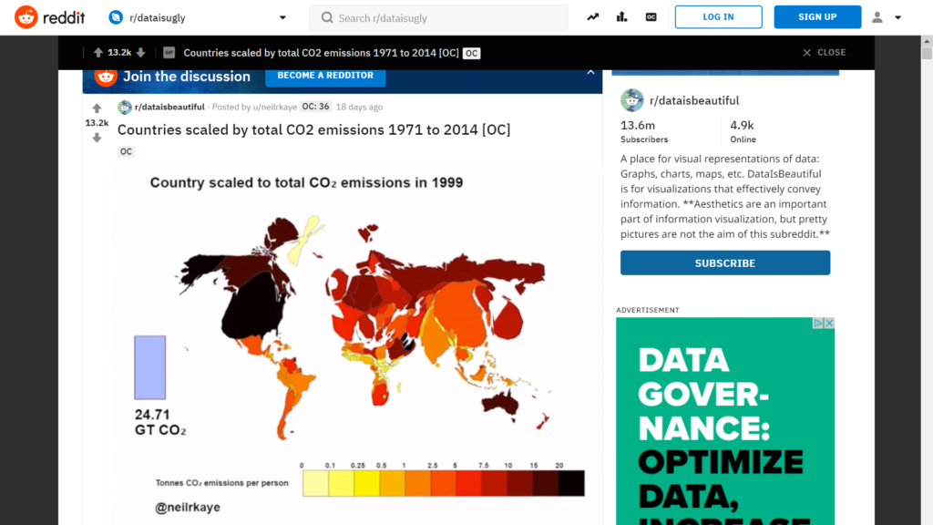
Cartograms are “map-like diagrams…which may purposefully distort map areas or represent them in stylized form, for example as equal-sized squares (Claus O. Wilke, Fundamentals of Data Visualization, Chapter 15, https://serialmentor.com/dataviz/geospatial-data.html#geospatial-data).” Cartograms are utilized with datasets that have a connection to a physical location. Cartograms are most effective when the data one wants to visualize is best represented in correlation/connection to its location in the physical world, but in circumstances in which maintaining the geographical accuracy of a standard map may threaten to distort the data being visualized. Cartograms can be designed to represent a comparative snapshot of a particular moment in time, or to illustrate comparative changes over time (see the Reddit example below). While the cartogram does not rely on a drawn map in order to organize data, the features of the created charts should bear a resemblance to the physical features of the associated geospatial locations. Cartograms are not very effective at displaying data that has no connection or correlation to a physical location, though there are ways in which non-geospatial data charts can be embedded within a cartogram in order to facilitate comparisons of data geographically.
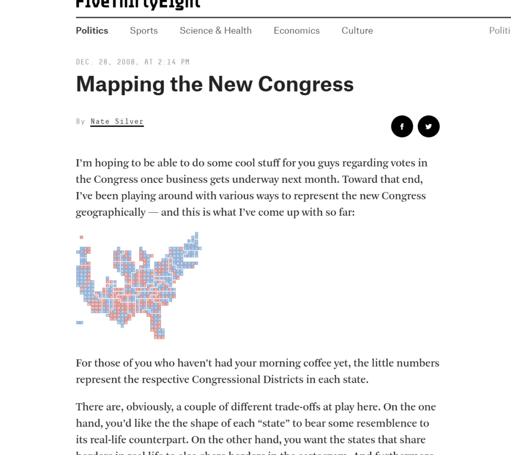
An example of an effective cartogram (more precisely, a cartogram heat map) can be viewed at the Five Thirty-Eight blog. The visualization depicts the composition of the newly-elected U.S. House of Representatives based upon party affiliation. The cartogram consists of 435 two dimensional squares of equal size. Each square within the chart represents a congressional district with the number at center of the block denoting which district. Because congressional apportionment is based upon population, and each representative represents roughly the same number of constituents, it makes sense to represent each district equally. Blue squares denote Democratically-held seats while red squares signify those districts represented by Republicans. Districts are grouped by state and placed in rough geospatial location to the positioning of that state on a U.S. map. The chart thus visually resembles the physical features of the United States. Lower populations in states along the Great Plains and Rocky Mountains result in some deformity in relation to a U.S. Map (Montana, North and South Dakota, and Wyoming, for example, only have 1 representative each, which reduces the size of their presence on the cartogram in comparison to the geographic area they occupy). Similarly, areas of high population density, such as New York City, occupy a significantly larger space on the cartogram than their geographic area. Despite the distortions, the visualization is quite easy to interpret with minimal explanation being required. This cartogram is useful in assisting analysis of regional strongholds for both the Republican and Democratic parties (with blue squares dominating in the Northeast and West Coast, and red concentrations across the Southeast and Plains States).
Histograms were created in the late 19th century by Karl Pearson (see https://flowingdata.com/2014/02/27/how-to-read-histograms-and-use-them-in-r/) and illustrate the distribution of a particular set of data over a period of time (or some other established interval). In a histogram, numerical data is separated into “bins” of the same type of data. Each bin is then displayed adjacent to other bins. This type of visualization is particularly useful to denote concentrations within a dataset as well as gaps or unusual values (extreme high or low concentrations for example).
While similar to bar graphs in appearance, histograms interpret data very differently. While bar graphs illustrate and quantify categorical types of data in a side-by-side correlation, histograms depict the distribution of particular types of data over a continuous variable, such as time (https://flowingdata.com/2014/02/27/how-to-read-histograms-and-use-them-in-r/).
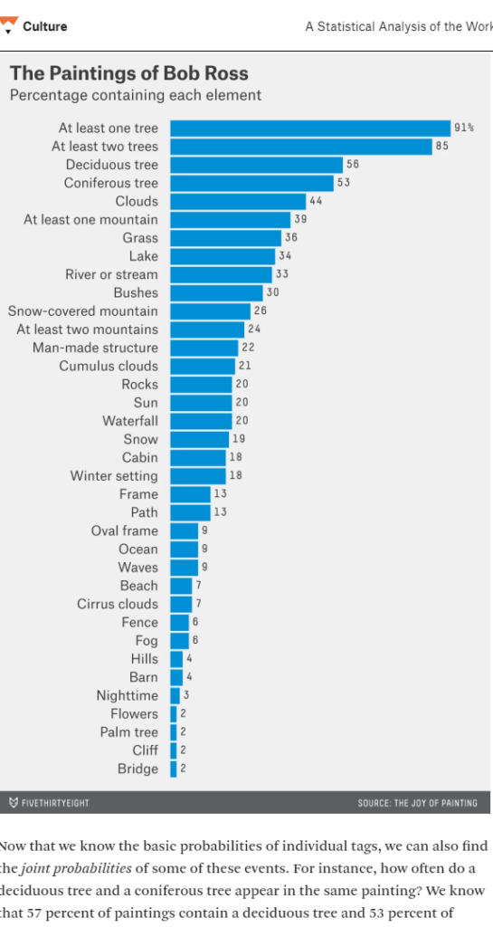
(https://fivethirtyeight.com/features/a-statistical-analysis-of-the-work-of-bob-ross/)
The Five Thirty-eight’s histogram analysis of the paintings of artist Bob Ross, which was featured in the assigned essay “Exploring Histograms” by Aran Lunzer and Ameila McNamara (https://tinlizzie.org/histograms/) examines paintings created by Ross over the course of 403 episodes of his PBS television show, “The Joy of Painting” between 1983 and 1994. In order to create the histogram, the data binned features in Bob Ross’ artwork (trees, mountains, clouds, etc.) to visually depict distributions of each feature.
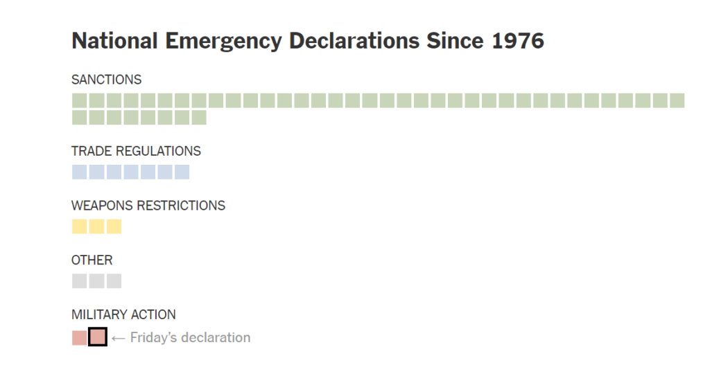
An example of a modified histogram appeared within the last week in the New York Times in the context of an article discussing the use of presidential emergency declarations since 1976 (https://www.nytimes.com/interactive/2019/02/15/us/list-of-national-emergencies.html). The histogram depicts 59 National Emergency Declarations since Congress enacted the legislation authorizing such declarations in 1976. Each declaration is represented by a square of equal size. The declarations are “binned” (divided) by type of emergency, with each type represented by a unique color. Among the types of emergency declarations issued by U.S. presidents since the Carter Administration, the New York Times article has grouped these declarations as sanctions (44), trade regulations (7), weapons restrictions (3), military action (2), and other (3). One square within the military action cluster is highlighted with a black border and labelled “Friday’s declaration.” The purpose of this histogram is to visually demonstrate the relative exceptionality of the current administration’s decision to enact an emergency declaration involving military action (the use of Department of Defense funding and personnel for the construction of a border wall). Prior to this February, the only other time military action had been authorized by a president under this legislation was in response to the September 11, 2001, attacks. The decision by the graphic’s creator to represent each declaration of a national emergency as a unique square as opposed to solid bars for each bin was clearly done in order to be able to call out the most recent emergency for analysis and public debate. Because the data is organized into bins determined by the creator, histogram data can be manipulated or distorted in an effort to better support one’s argument.

3 Comments
Maeve Kane
Remember that this needs a read more cut after the first one or two paragraphs!
amnoble
There is a cut with the image and paragraph 1 when I open it on my work browser (Chrome). Does it not show up elsewhere?
Maeve Kane
No, your post is fine, I’m just dumb and got my tabs mixed up. My comment was meant for a different post, sorry about that!