Uncategorized
-
Networks
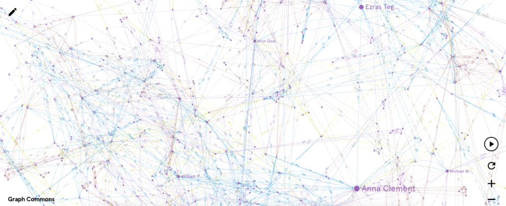
1: Over time, individual clusters are brought together with other clusters through connectors. What interested me was that while some individuals were strengthening their networks smaller clusters were forming outside the main networks. Over time these are slowly brought into the larger network through connectors, like William Corry Esqr. Other big connectors were John Wemp, Esras Teganderasse, Aron Oseragighte and Anna Clement. Some of these brought groups together then their number of connections decreased relative to those around them. There names began to blend in, with some exceptions, like Anna Clement and Esras Teganderasse and Michael Montour who seem to be who are holding the two large networks together.
-
Networks
The network grows as more years are introduced. However, this also means that the web of people becomes more difficult to read. Luckily, the years are separated into colors which means it is slightly easier to pick out connections. Interestingly, many years start a new sub-group of people and most do not have connections to the years prior. I consider these groups the outliers as they are not present on the graph when it’s zoomed in. This leads to a conclusion that new people must either be coming to town or joining the congregation each year, regardless of if they know someone. The biggest nodes on the map belong to John Wemp and Mary Butler, who are also connected. I do not necessarily understand why this is but both have many connections on the map from various years and those connections make more connections as well.
-
Networks
Over time, the network gets bigger and more connections are added. Some major connectors I’ve found are Esras Sr., Anna and Joseph Clement, Cornelius Thanighwanege, Abraham Canostens Peterse, and Seth Sietstarare Karihoge.
The network compared by betweenness seems to have less connections than the one sized by degree. There are two main groups which only have a few connections between them. There are also a lot of smaller groups that have four to ten people in them, and they don’t connect to either of the larger two groups.
There seems to be a lot less large nodes when sized by betweenness. The network filtered by year provides a lot more major connectors than when it is filtered by betweenness. Many of the larger nodes when sized by betweenness are the same people as when it’s filtered by year.
The patterns formed by clustering seem like that don’t have much that is similar with individuals with high betweenness centrality. The only person in common that I saw was Anna Clement. This could have been because I missed some of the other major individuals when they were grouped in other ways, or that they weren’t as major when grouped differently.
The patterns formed by clustering look similar to the ones formed when the data was filtered by year. While the patterns compared by betweenness had two major groups that were clearly split, the patterns with clustering overlap a lot and don’t have any groups that are clearly split. It looks very similar to the way the patterns were when it was filtered by year.
-
Networks: Jeffrey Aldrich
In this week’s Networks tutorial there are many interesting factors that stand out while studying the edges between the different members of the church congregation.
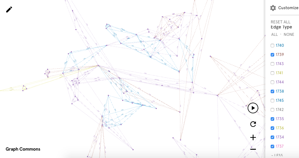
The first question to address is how these networks of church members change over the years 1735-1745. The first two major variables to assess over time are the change in the quantity of networks and the change in the overall size of each network throughout the decade. There are essentially three primary phases in the data set. The first is at 1734-1735. This period is represented by a minute number of networks with a minimal number of edges and nodes. The second phase runs from 1736-1739. At this point, two larger networks have formed with smaller networks scattered throughout the periphery. The number of edges and nodes has also largely increased. Lastly, the final phase is from 1740-1745. At this point the two larger networks, seen in the previous phase, have joined together, and there are several, smaller networks throughout the periphery. This phase also contains the largest number of nodes and edges.
-
Networks Project
In analyzing the church congregation networks between 1735-45, the program gives the viewer the opportunity to view the vast interweaving connections between members of the congregation. In viewing the network through the filter of time, selecting subsequent years allows the viewer to witness the evolution of the complex network that existed by 1745. The first two years of the congregation consisted primarily of small, detached networks. However, as the years progress, networks become more complex: new networks are created, existent networks grow in size, and previously disconnected networks become intertwined. One benchmark year in the growth of the congregational network was 1738, when significant connections between disjointed networks were created.
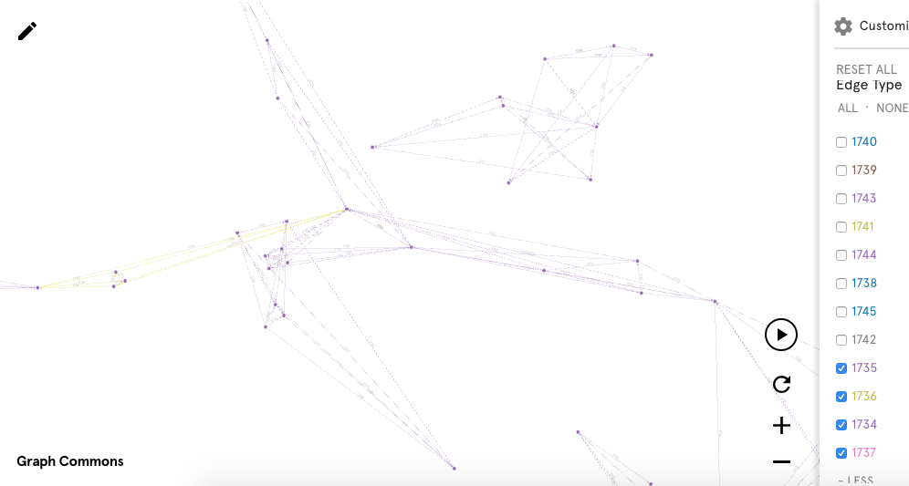
1737 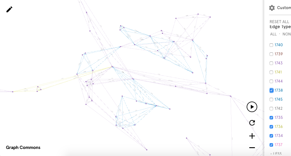
1738
The following year, 1739, was marked by increasing connections between “far away” or largely disjointed networks.
When measuring the networks by the betweenness centrality, the map becomes increasingly complex, with numerous connections across distinct nodes. These connections branch out from large “node centers” around individuals with a high degree of betweenness centrality: Anna Clement, Esras Sr, William Prentop Jr., Leut Burrows, Aron Oseragighte, and Ezras Teg are some of the more prominent figures in this view.
When returning to the network view based on degree centrality, many of these figures remain prominent with a number of connections to other individuals, including Anna Clement, Esras Sr, and Aron Oseragighte. However, there are others such as Mary Butler and William Mills who do not appear to have as high of a degree of betweenness centrality.
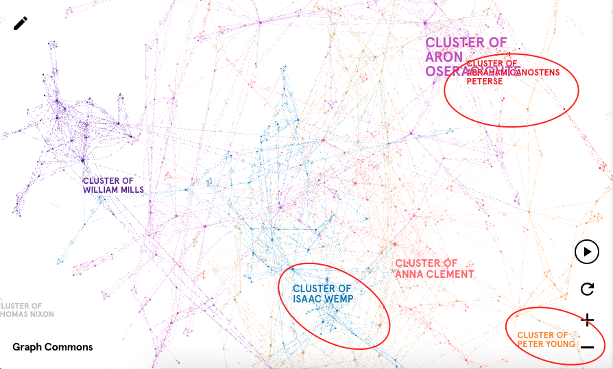
When viewing clustering patterns, many of the figures who exhibit a high degree of betweenness centrality and/or degree centrality have clusters build around them; Oseragighte, Clement, and Mills are a few examples of this. However, several other clusters form around individuals not prominent in these other views, notably Peter Young, Isaac Wemp, Abraham Canostens Peterse, and Cornelius Brown.
Overall, viewing these different elements of the network gives the audience an insight into potentially important or well-connected individuals within the congregation. It highlights those that are perhaps more obviously within the realm of influence or significance, as well as those whose connections might be more abstract or subtle.
-
Networks
By Jesse Aragona
- As you add years into the network, family connections continue to develop and grow as more are people are born. The major connectors who cause more and more intertwined networks tend to be both the original founders of the network and offspring they inevitably have. As children from different families intermarry, more and more connections develop between groups eventually creating a vast inter connected network especially with the sample data set.
- The betweeness centrality is used to find the influence a particular node has over the larger graph, judging it by what connections it helps create where as filtering by degree is simply designed to find the largest amount of connections. While there does tend to be some overlap, those found by filtering by centrality are not necessarily the same as those who have the most connections when filtered by year. While these tools can produce similar results its important to recognize the differences between these two approaches, as commonality doesn’t necessarily produce exact results.
- Patterns formed by clustering finds individual who have the same connections, grouping them into a class. They tend to be better represented then those found filtering by year, as well as more closely related. Using this method we can better compare individuals, allowing us to see best who relates to who and how.
-
Intro to Networks
When looking at only 1734, Mary Butler seems to be well-connected with other nodes. Her connections grow stronger in 1735. Once the data for 1740 is included, Mary remains the largest node, therefore the most connected, but the diagram grows increasingly complex. Once the data for every available year is included, Mary Butler is still the largest node.
-
Heat Maps and Dendrograms

There’s a weird amount of heatmap memes on the Internet Heat Maps
A heat map is a way to visualize data that is reliant on color variation. All heat maps require a legend to show what each color means. It can show labeled categorical data or qualitative data so long as it corresponds with a color. While some he maps may have specific colors, others can cover a range. This kind of heat map works best with quantitative, continuous data that allows for a range of possibilities, such as temperature.
-
Choropleth and Heat Maps
Choropleth map uses shading and color variation to display data on a specific geographic location. This type of data visualization is most often associated with the display of population densities, income distribution, and election results. Choropleth maps are best at displaying density. By using either varying shades of a single color, transitions along a color scale, or discrete color blocks, Choropleth maps take advantage of contrast to display data on a geographic boundary.
-
Horizon Graphs and Small Multiples
Horizon Graph
A horizon graph is a chart that utilizes a diverging color scale, where either end of a data sequence is represented with different opaque colors that stratigraphically become more translucent and similar to the opposing color as the data reaches a start value, to showcase the different values within a dataset.
To create a horizon graph, one begins with a simple line graph that can go both positive and negative along the X or Y axis. After a line has been plotted, then a different color is used to represent each group of data within a given range. Then, all of the different color categories are re-plotted with only positive values on the graph at the axis.
An excellent example of a horizon graph can be found at flowingdata.com. In this example, the author uses a horizon graph to show the fluctuating price of bacon from 1990 to 2015. These three steps, below, show how the author shifted the data visualization from a line graph to a horizon graph: